 (Fig. 1a)
 (Fig. 1b)
In gradient descent we start at some point on the error function defined over the weights, and attempt to move to the global minimum of the function. In the simplified function of Fig 1a the situation is simple. Any step in a downward direction will take us closer to the global minimum. For real problems, however, error surfaces are typically complex, and may more resemble the situation shown in Fig 1b. Here there are numerous local minima, and the ball is shown trapped in one such minimum. Progress here is only possible by climbing higher before descending to the global minimum.
 (Fig. 1a)
 (Fig. 1b)
We have already mentioned one way to escape a local minimum: use online learning. The noise in the stochastic error surface is likely to bounce the network out of local minima as long as they are not too severe.

| (1) |
where 0 < m < 1 is a new global parameter which must be determined by trial and error. Momentum simply adds a fraction m of the previous weight update to the current one. When the gradient keeps pointing in the same direction, this will increase the size of the steps taken towards the minimum. It is otherefore often necessary to reduce the global learning rate µ when using a lot of momentum (m close to 1). If you combine a high learning rate with a lot of momentum, you will rush past the minimum with huge steps!
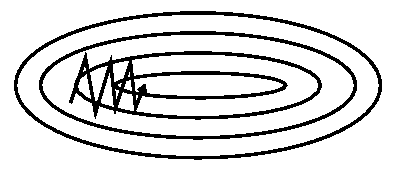
When the gradient keeps changing direction, momentum will smooth out the variations. This is particularly useful when the network is not well-conditioned. In such cases the error surface has substantially different curvature along different directions, leading to the formation of long narrow valleys. For most points on the surface, the gradient does not point towards the minimum, and successive steps of gradient descent can oscillate from one side to the other, progressing only very slowly to the minimum (Fig. 2a). Fig. 2b shows how the addition of momentum helps to speed up convergence to the minimum by damping these oscillations.
 (Fig. 2a)
 (Fig. 2b)
To illustrate this effect in practice, we trained 20 networks on a simple problem (4-2-4 encoding), both with and without momentum. The mean training times (in epochs) were
| momentum | Training time |
|---|---|
| 0 | 217 |
| 0.9 | 95 |
Bold Driver
A useful batch method for adapting the global learning rate µ is the bold driver algorithm. Its operation is simple: after each epoch, compare the network's loss E(t) to its previous value, E(t-1). If the error has decreased, increase µ by a small proportion (typically 1%-5%). If the error has increased by more than a tiny proportion (say, 10-10), however, undo the last weight change, and decrease µ sharply - typically by 50%. Thus bold driver will keep growing µ slowly until it finds itself taking a step that has clearly gone too far up onto the opposite slope of the error function. Since this means that the network has arrived in a tricky area of the error surface, it makes sense to reduce the step size quite drastically at this point.
Annealing
Unfortunately bold driver cannot be used in this form for online learning: the stochastic fluctuations in E(t) would hopelessly confuse the algorithm. If we keep µ fixed, however, these same fluctuations prevent the network from ever properly converging to the minimum - instead we end up randomly dancing around it. In order to actually reach the minimum, and stay there, we must anneal (gradually lower) the global learning rate. A simple, non-adaptive annealing schedule for this purpose is the search-then-converge schedule
| µ(t) = µ(0)/(1 + t/T) | (2) |
Its name derives from the fact that it keeps µ nearly constant for the first T training patterns, allowing the network to find the general location of the minimum, before annealing it at a (very slow) pace that is known from theory to guarantee convergence to the minimum. The characteristic time T of this schedule is a new free parameter that must be determined by trial and error.
Local Rate Adaptation
If we are willing to be a little more sophisticated, we go a lot further than the above global methods. First let us define an online weight update that uses a local, time-varying learning rate for each weight:
|
| (3) |
The idea is to adapt these local learning rates by gradient descent, while simultaneously adapting the weights. At time t, we would like to change the learning rate (before changing the weight) such that the loss E(t+1) at the next time step is reduced. The gradient we need is
|
| (4) |
Ordinary gradient descent in µij, using the meta-learning rate q (a new global parameter), would give
|
| (5) |
We can already see that this would work in a similar fashion to momentum: increase the learning rate as long as the gradient keeps pointing in the same direction, but decrease it when you land on the opposite slope of the loss function.
Problem: µij might become negative! Also, the step size should be proportional to µij so that it can be adapted over several orders of magnitude. This can be achieved by performing the gradient descent on log(µij) instead:
|
| (6) |
Exponentiating this gives

| (7) |
where the approximation serves to avoid an expensive exp function call. The multiplier is limited below by 0.5 to guard against very small (or even negative) factors.
Problem: the gradient is noisy; the product of two of them will be even noisier - the learning rate will bounce around a lot. A popular way to reduce the stochasticity is to replace the gradient at the previous time step (t-1) by an exponential average of past gradients. The exponential average of a time series u(t) is defined as
|
| (8) |
where 0 < m < 1 is a new global parameter.
Problem: if the gradient is ill-conditioned, the product of two gradients will be even worse - the condition number is squared. We will need to normalize the step sizes in some way. A radical solution is to throw away the magnitude of the step, and just keep the sign, giving
|
| (9) |
where r = eq. This works fine for batch learning, but...
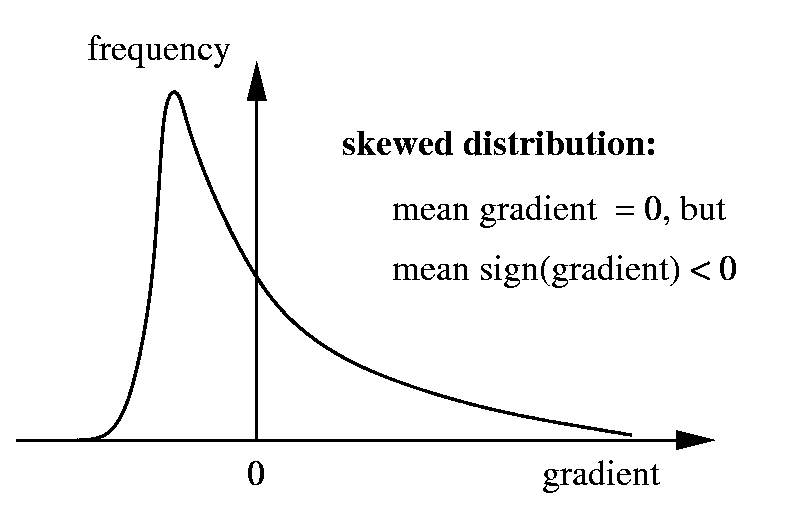
 (Fig. 3)
Problem: Nonlinear normalizers such as the sign function lead to
systematic errors in stochastic gradient descent (Fig. 3): a skewed but
zero-mean gradient distribution (typical for stochastic equilibrium) is
mapped to a normalized distribution with non-zero mean. To avoid the
problems this is casuing, we need a linear normalizer for online learning.
A good method is to divide the step by
![]() ,
an exponential average of the squared gradient. This gives
,
an exponential average of the squared gradient. This gives

| (10) |
Problem: successive training patterns may be correlated, causing the product of stochastic gradients to behave strangely. The exponential averaging does help to get rid of short-term correlations, but it cannot deal with input that exhibits correlations across long periods of time. If you are iterating over a fixed training set, make sure you permute (shuffle) it before each iteration to destroy any correlations. This may not be possible in a true online learning situation, where training data is received one pattern at a time.
To show that all these equations actually do something useful, here is a typical set of online learning curves (in postscript) for a difficult benchmark problem, given either uncorrelated training patterns, or patterns with strong short-term or long-term correlations. In these figures "momentum" corresponds to using equation (1) above, and "s-ALAP" to equation (10). "ALAP" is like "s-ALAP" but without the exponential averaging of past gradients, while "ELK1" and "SMD" are more advanced methods (developed by one of us).