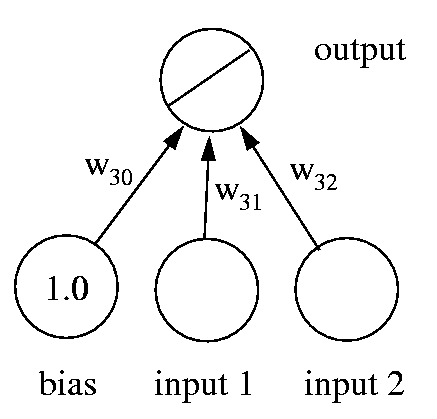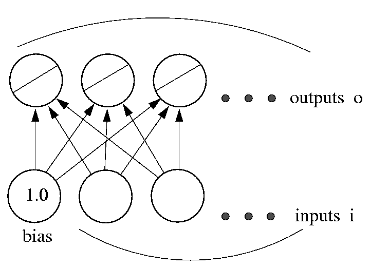

Similarly, we may want to predict more than one variable from the data that we're given. This can easily be accommodated by adding more output units (Fig. 2). The loss function for a network with multiple outputs is obtained simply by adding the loss for each output unit together. The network now has a typical layered structure: a layer of input units (and the bias), connected by a layer of weights to a layer of output units.

| 
|
| (Fig. 1) | (Fig. 2) |
In order to train neural networks such as the ones shown above by gradient descent, we need to be able to compute the gradient G of the loss function with respect to each weight wij of the network. It tells us how a small change in that weight will affect the overall error E. We begin by splitting the loss function into separate terms for each point p in the training data:
 | (1) |
where o ranges over the output units of the network. (Note that we use the superscript p to denote the training point - this is not an exponentiation!) Since differentiation and summation are interchangeable, we can likewise split the gradient into separate components for each training point:
 | (2) |
In what follows, we describe the computation of the gradient for a single data point, omitting the superscript p in order to make the notation easier to follow.
First use the chain rule to decompose the gradient into two factors:
 | (3) |
The first factor can be obtained by differentiating Eqn. 1 above:
 | (4) |
Using  , the second factor becomes
 | (5) |
Putting the pieces (equations 3-5) back together, we obtain
 | (6) |
To find the gradient G for the entire data set, we sum at each weight the contribution given by equation 6 over all the data points. We can then subtract a small proportion µ (called the learning rate) of G from the weights to perform gradient descent.
The algorithm terminates once we are at, or sufficiently near to, the minimum of the error function, where G = 0. We say then that the algorithm has converged.
- Initialize all weights to small random values.
- REPEAT until done
- For each weight wij set

- For each data point (x, t)p
- set input units to x
- compute value of output units
- For each weight wij set
- For each weight wij set

In summary:
general case linear network Training data (x,t) (x,t) Model parameters w w Model y = g(w,x) Error function E(y,t) Gradient with respect to wij - (ti - yi) yj Weight update rule
The Learning Rate
An important consideration is the learning rate µ, which determines by how much we change the weights w at each step. If µ is too small, the algorithm will take a long time to converge (Fig. 3).
(Fig. 3)
Conversely, if µ is too large, we may end up bouncing around the error surface out of control - the algorithm diverges (Fig. 4). This usually ends with an overflow error in the computer's floating-point arithmetic.
(Fig. 4)
Batch vs. Online Learning
Above we have accumulated the gradient contributions for all data points in the training set before updating the weights. This method is often referred to as batch learning. An alternative approach is online learning, where the weights are updated immediately after seeing each data point. Since the gradient for a single data point can be considered a noisy approximation to the overall gradient G (Fig. 5), this is also called stochastic (noisy) gradient descent.
(Fig. 5)
Online learning has a number of advantages:
These advantages are, however, bought at a price: many powerful optimization techniques (such as: conjugate and second-order gradient methods, support vector machines, Bayesian methods, etc.) - which we will not talk about in this course! - are batch methods that cannot be used online. (Of course this also means that in order to implement batch learning really well, one has to learn an awful lot about these rather complicated methods!)
- it is often much faster, especially when the training set is redundant (contains many similar data points),
- it can be used when there is no fixed training set (new data keeps coming in),
- it is better at tracking nonstationary environments (where the best model gradually changes over time),
- the noise in the gradient can help to escape from local minima (which are a problem for gradient descent in nonlinear models).
A compromise between batch and online learning is the use of "mini-batches": the weights are updated after every n data points, where n is greater than 1 but smaller than the training set size.
In order to keep things simple, we will focus very much on online learning, where plain gradient descent is among the best available techniques. Online learning is also highly suitable for implementing things such as reactive control strategies in adapative agents, and should thus fit in well with the rest of your course.
goto top of page [Next: Multi-layer networks]
[Back to the first page]