 |
(1) |
In the previous example we used a network with two hidden units. Just by looking at the data, it was possible to guess that two tanh functions would do a pretty good job of fitting the data. In general, however, we may not know how many hidden units, or equivalently, how many weights, we will need to produce a reasonable approximation to the data. Furthermore, we usually seek a model of the data which will give us, on average, the best possible predictions for novel data. This goal can conflict with the simpler task of modelling a specific training set well. In this section we will look at some techniques for preventing our model becoming too powerful (overfitting). In the next, we address the related question of selecting an appropriate architecture with just the right amount of trainable parameters.
 |
(1) |
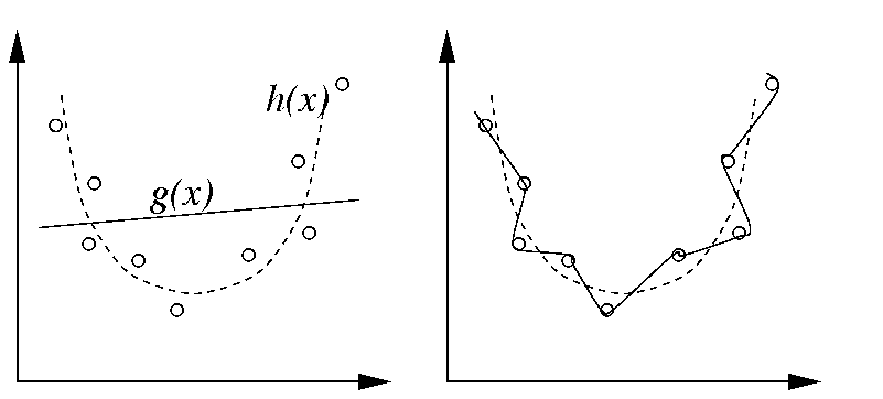
In the left hand panel we try to fit the points using a function g(x) which has too few parameters: a straight line. The model has the virtue of being simple; there are only two free parameters. However, it does not do a good job of fitting the data, and would not do well in predicting new data points. We say that the simpler model has a high bias.

The right hand panel shows a model which has been fitted using too many free parameters. It does an excellent job of fitting the data points, as the error at the data points is close to zero. However it would not do a good job of predicting h(x) for new values of x. We say that the model has a high variance. The model does not reflect the structure which we expect to be present in any data set generated by equation (1) above.
Clearly what we want is something in between: a model which is powerful enough to represent the underlying structure of the data (h(x)), but not so powerful that it faithfully models the noise associated with this particular data sample.
The bias-variance trade-off is most likely to become a problem if we have relatively few data points. In the opposite case, where we have essentially an infinite number of data points (as in continuous online learning), we are not usually in danger of overfitting the data, as the noise associated with any single data point plays a vanishingly small role in our overall fit. The following techniques therefore apply to situations in which we have a finite data set, and, typically, where we wish to train in batch mode.

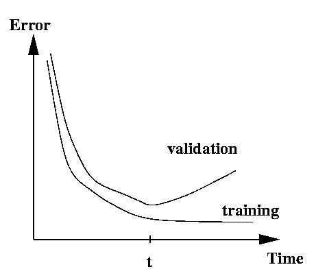
One detail of note when using early stopping: if we wish to test the trained network on a set of independent data to measure its ability to generalize, we need a third, independent, test set. This is because we used the validation set to decide when to stop training, and thus our trained network is no longer entirely independent of the validation set. The requirements of independent training, validation and test sets means that early stopping can only be used in a data-rich situation.
 |
(2) |
One possible form of the regularizer comes from the informal observation that an over-fitted mapping with regions of large curvature requires large weights. We thus penalize large weights by choosing
 |
(3) |
Using this modified error function, the weights are now updated as
 |
(4) |
where the right hand term causes the weight to decrease as a function of its own size. In the absence of any input, all weights will tend to decrease exponentially, hence the term "weight decay".
 instead.
At first, this may seem a rather odd thing to do: to deliberately corrupt ones own data. However, perhaps you can see that it will now be difficult for the network to approximate any specific data point too closely. In practice, training with added noise has indeed been shown to reduce overfitting and thus improve generalization in some situations.
If we have a finite training set, another way of introducing noise into the training process is to use online training, that is, updating weights after every pattern presentation, and to randomly reorder the patterns at the end of each training epoch. In this manner, each weight update is based on a noisy estimate of the true gradient.